 |
Logbook
(07-04-2025)
Static problems
|


|
|
Logbook
(07-04-2025)
Static problems
|
|
Solves static scalar boundary value problem. More...
#include <static_scalar_solver.hpp>
Public Member Functions | |
| Solver (unsigned int p, unsigned int mapping_degree, unsigned int type_of_pde_rhs, std::string fname="data", const Function< dim > *exact_solution=nullptr, bool axisymmetric=false, bool vector_potential=false, bool print_time_tables=false, bool project_exact_solution=false, bool write_higher_order_cells=false) | |
| The only constructor. More... | |
| virtual void | make_mesh ()=0 |
| Initializes the data member StaticScalarSolver::Solver::triangulation. More... | |
| virtual void | fill_dirichlet_stack ()=0 |
| Initializes the data member StaticScalarSolver::Solver::dirichlet_stack. More... | |
| virtual void | solve ()=0 |
| Solves the system of linear equations. | |
| void | setup () |
| Initializes system matrix and the right-hand side vector, etc. More... | |
| void | assemble () |
| Assembles the system matrix and the right-hand side vector. | |
| void | compute_error_norms () |
| Computes error norms. | |
| void | project_exact_solution_fcn () |
| Projects exact solution. More... | |
| void | save () const |
| Saves simulation results into a vtk or vtu file. More... | |
| void | save_matrix_and_rhs_to_csv (std::string fname) const |
| Saves the system matrix and the right-hand side into a csv file. More... | |
| void | clear () |
| Releases computer memory associated with the system matrix and right-hand side. | |
| const Triangulation< dim > & | get_tria () const |
| Returns a reference to triangulation. | |
| const DoFHandler< dim > & | get_dof_handler () const |
| Returns a reference to dof handler. | |
| const Vector< double > & | get_solution () const |
| Returns a reference to the solution. | |
| unsigned int | get_n_cells () const |
| Returns the number of active cells in the mesh. | |
| unsigned int | get_n_vertices () const |
| Returns the number of vertices. | |
| unsigned int | get_n_used_vertices () const |
| Returns the number of used vertices. | |
| unsigned int | get_n_lines () const |
| Returns the number of lines. | |
| unsigned int | get_n_dofs () const |
| Returns the total amount of the degrees of freedom. | |
| unsigned int | get_type_of_pde_rhs () const |
Returns the value of type_of_pde_rhs. | |
| double | get_L2_norm () const |
| Returns \(L^2\) error norm. | |
| double | get_H1_norm () const |
| Returns \(H^1\) error norm. | |
| double | get_Linfty_norm () const |
| Returns \(L^{\infty}\) error norm. | |
| unsigned int | get_mapping_degree () const |
| Returns degree of the interpolating Lagrange polynomials used for mapping from the reference cell to the real mesh cell and back. | |
| void | run () |
| Runs the simulation. More... | |
Protected Attributes | |
| std::map< types::boundary_id, const Function< dim > * > | dirichlet_stack |
| A map that contains pairs of boundary IDs and the corresponding Dirichlet boundary conditions. More... | |
| Triangulation< dim > | triangulation |
| The mesh. | |
| const FE_Q< dim > | fe |
| The finite elements. | |
| DoFHandler< dim > | dof_handler |
| The degrees-of-freedom handler. | |
| Vector< double > | solution |
| The solution vector, i.e., degrees of freedom yielded by the simulation. | |
| Vector< double > | projected_exact_solution |
| The projected exact solution vector. | |
| AffineConstraints< double > | constraints |
| The constraints associated with the Dirichlet boundary conditions. | |
| SparsityPattern | sparsity_pattern |
| The sparsity pattern of the system matrix. | |
| SparseMatrix< double > | system_matrix |
| The system matrix. | |
| Vector< double > | system_rhs |
| The system right-hand side vector. | |
| double | L2_norm |
| The \(L^2\) error norm. | |
| double | Linfty_norm |
| The \(L^{\infty}\) error norm. | |
| double | H1_norm |
| The \(H^1\) error semi-norm. | |
Solves static scalar boundary value problem.
Implements the following recipes:
This class template is intended to be a general solver for problems in electro- and magnetostatics that can be formulated in therms of the electrostatic scalar potential, \(\Phi\), total magnetostatic scalar potential, \(\Psi\), reduced magnetostatic scalar potential, \(\Theta\), two-dimensional magnitude of vector potential, \(A\), and scaled two-dimensional magnitude of vector potential, \(A'\). It can also be used to solve for the current vector potential, \(T\), in planar two-dimensional problems. The calculated potential is saved in a vtk file, see function save() for more details. The Bossavit's diagrams below illustrate the partial differential equations that can be solved with a help of this class template. Note, that in all cases listed below the potential belongs to the \(H(\text{grad})\) function space, i.e., is modeled by the FE_Q finite elements.
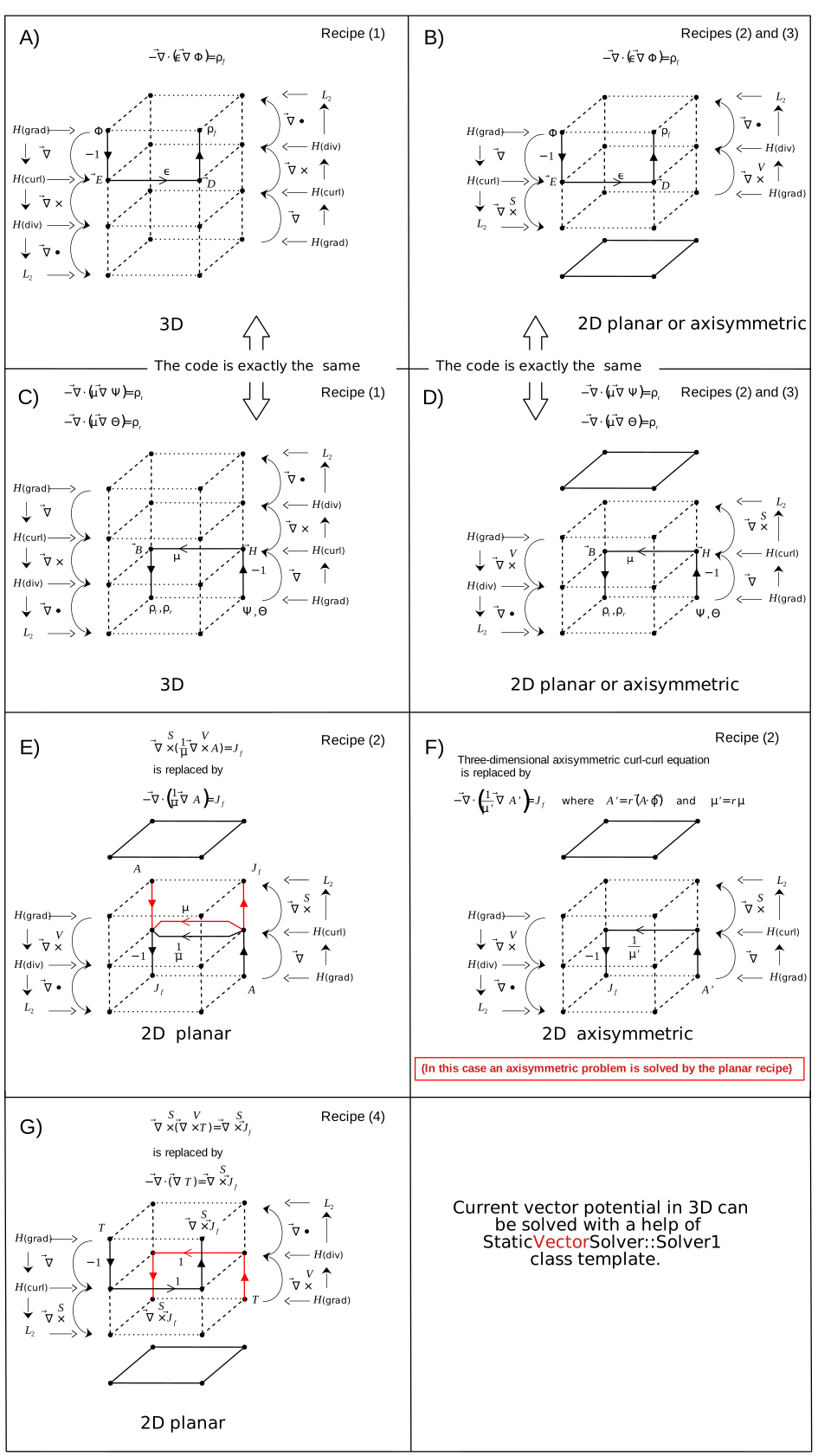
The table below lists the recommended settings for switching between different types of problems. The letters in the first column of the table correspond to the seven diagrams above. The dim parameter is the input parameter of the class template. The other three parameters, type_of_pde_rhs, axisymmetric, and vector_potential, are passed as input parameters to the constructor of the class.
| Insert | dim | type_of_pde_rhs | axisymmetric | vector_potential |
|---|---|---|---|---|
| A), C) | 3 | 0 or 1 | false | false |
| B), D) | 2 | 0 or 1 | true or false | false |
| E) | 2 | 0 or 1 | false | true |
| F) | 2 | 0 or 1 | false | true |
| G) | 2 | 2 or 3 | false | true |
A user of this class is supposed to do the following.
type_of_pde_rhs=2), StaticScalarSolver::Gamma, StaticScalarSolver::RobinRhs, and StaticScalarSolver::FreeSurfaceCharge, StaticScalarSolver::Weight.The boundaries of the mesh must be labeled such that the boundary_id member function of a face object returns the corresponding boundary ID. The boundary ID's must obey the following convention.
value_list(...) methods of the class templates StaticScalarSolver::RobinRhs and StaticScalarSolver::Gamma.The constructor's argument type_of_pde_rhs switches the operation of the class template between following four modes:
type_of_pde_rhs = 1. In this mode the right-hand side of the partial differential equation is assumed to be a scalar field. Let us for the sake of illustration assume that we are computing the electric scalar potential, \(\Phi\), and that the right-hand side is the free-charge density, \(\rho_f\). Then the partial differential equation reads \[ - \vec{\nabla} \cdot \big( \epsilon \vec{\nabla} \Phi \big)= \rho_f. \]
The corresponding integral in the variational formulation reads\[ \iiint_{\Omega} \rho_f \Phi dV \]
in three dimensions and\[ \iint_{\Omega} \rho_f \Phi dS \]
in two dimensions. In this mode the values of \(\rho_f\) at quadrature points are computed by calling StaticScalarSolver::PdeRhs::value_list.type_pde_rhs = 0. Setting type_pde_rhs = 0 is the same as setting type_pde_rhs = 1 and \(\rho_f = 0\). In this mode algorithm saves some time on calling StaticScalarSolver::PdeRhs::value_list and evaluating the two integrals above.type_pde_rhs = 3. In this mode the class template computes the two-dimensional current vector potential, \(T\), by solving the following partial differential equation: \[ - \vec{\nabla} \cdot \big(\vec{\nabla} T \big)= \vec{\nabla} \overset{S}{\times}\vec{J}_f. \]
This mode works only in two dimensions (the class template StaticVectorSolver::Solver1 must be used for calculating the current vector potential in three dimensions). The following two integrals represent the right-hand side of the partial differential equation in the functional:\[ \iint_{\Omega}\vec{J}_f\cdot\bigg(\vec{\nabla}\overset{V}{\times}T\bigg)dS- \underbrace{\oint_{\Gamma} \vec{J}_f \cdot \bigg(\hat{n} \overset{V}{\times} T \bigg) dl}_{\text{Boundary integral}}. \]
That is to say, in this mode the source on the right-hand side of the partial differential equation is not a scalar field (such as \(\rho_f\)), but a two-dimensional vector field, \(\vec{J}_f\). The class template calls an object of the type StaticScalarSolver::PdeRhsCvp to evaluate the values of \(\vec{J}_f\) at quadrature points.type_pde_rhs = 2. There is only one difference between this mode and the mode type_pde_rhs = 3. In this mode the boundary integral, see above, is not computed. This can save simulation time if \(\vec{J}_f = 0\) on the boundary by definition of the problem, see (cvp-ii) numerical experiment for an example.This class template utilizes the WorkStream technology of deal.II. The amount of threads used can be limited as the following
Definition at line 236 of file static_scalar_solver.hpp.
|
inline |
The only constructor.
| [in] | p | - The degree of the interpolating Lagrange polynomials in finite elements that model the potential. |
| [in] | mapping_degree | - The degree of the interpolating Lagrange polynomials used for mapping. Setting it to 1 will do in the most of the cases. Note, that it makes sense to attach a meaningful manifold to the triangulation if this parameter is greater than 1. |
| [in] | type_of_pde_rhs | - Switches between four modes of operation, see above. |
| [in] | fname | - The name of the output files without extension. |
| [in] | exact_solution | - Points to an object that describes the exact solution to the problem. It is needed for calculating error norms. It is a responsibility of the user to make sure that the object exists at the time of the execution of run() or compute_error_norms(). |
| [in] | axisymmetric | - If true, assumes that the problem is axisymmetric. If axisymmetric = true, dim must equal 2. |
| [in] | vector_potential | - If true, assumes that the problem is two-dimensional and formulated in terms of the magnitude of vector potential, \(A\), or in terms of the scaled magnitude of vector potential, \(A'\), or current vector potential, \(T\). If vector_potential = true, dim must equal 2. |
| [in] | print_time_tables | - If true, prints time tables on the screen. |
| [in] | project_exact_solution | - If true, projects the exact solution onto the space spanned by the Lagrange finite elements (FE_Q) and saves the result into the output file next to the solution. This may be useful for debugging purposes as a comparison between the projected exact solution and the solution to the boundary value problem can yield a hint on where to search for bugs. |
| [in] | write_higher_order_cells | - Switches between the two modes of operation of the save() function, see the description of save(). |
Definition at line 273 of file static_scalar_solver.hpp.
|
pure virtual |
Initializes the data member StaticScalarSolver::Solver::dirichlet_stack.
This function must be overridden by the user. It must initialize the stack of the Dirichlet boundary conditions. For example,
The boundary IDs must be odd numbers, see above the convention on the boundary IDs.
|
pure virtual |
Initializes the data member StaticScalarSolver::Solver::triangulation.
This function must be overridden by the user. It must generate or load the mesh, label the boundaries, and, if necessary, assign user IDs. This function is an ideal place for binding manifolds to the mesh. The last is a reasonable thing to do if mapping_degree > 1. The mesh must be stored in the data member of this class, StaticScalarSolver::Solver::triangulation.
| void StaticScalarSolver::Solver< dim, stage >::project_exact_solution_fcn |
Projects exact solution.
The mesh and the finite elements are the same as are used for the numerical solution of the boundary value problem. The exact solution will be saved in the output file next to the numerical solution to the boundary value problem. This function works properly only if the exact solution is submitted to the constructor via the input parameter exact_solution and project_exact_solution = true.
Definition at line 1284 of file static_scalar_solver.hpp.
|
inline |
Runs the simulation.
Executes the following member functions in a proper order: make_mesh(); fill_dirichlet_stack(); setup(); assemble(); solve(); project_exact_solution_fcn(); compute_error_norms(); save();
Definition at line 575 of file static_scalar_solver.hpp.
| void StaticScalarSolver::Solver< dim, stage >::save |
Saves simulation results into a vtk or vtu file.
The following data are saved:
The "L2norm", "H1seminorm", "LinftyNorm", and "ScalarFieldExact" are saved only if an exact solution is submitted to the constructor. Moreover, "ScalarFieldExact" is calculated and saved only if project_exact_solution = true.
If write_higher_order_cells = false, the name of the file is computed by appending ".vtk" to the string contained by the parameter fname passed to the constructor. The file can be inspected with a help of VisIt or Paraview. Higher-order cells are saved as regular quadrilaterals and hexahedra. If write_higher_order_cells = true, the name of the file is computed by appending ".vtu" to the string contained by the parameter fname. The data is saved preserving the higher-order cells. The file can be viewed with a help of Paraview version 5.5.0 or higher. VisIt cannot load higher-order cells.
Definition at line 1301 of file static_scalar_solver.hpp.
| void StaticScalarSolver::Solver< dim, stage >::save_matrix_and_rhs_to_csv | ( | std::string | fname | ) | const |
Saves the system matrix and the right-hand side into a csv file.
All the zeros are included into the csv files. This is a very dumb and inefficient way of saving sparse matrices. On the positive side - it is very easy and straightforward to read the csv files. This function may be useful for debugging. One can assemble the system on a coarse mesh (so there are a few mesh cells and the system matrix is small) and export the system matrix together with the right-hand side into another program such as Matlab or GNU Octave for an analysis.
| [in] | fname | - A stem of the names of the output files. The matrix will be saved into fname_matrix.csv file. The right-hand side will be save into fname_rhs.csv file. |
Definition at line 1346 of file static_scalar_solver.hpp.
| void StaticScalarSolver::Solver< dim, stage >::setup |
Initializes system matrix and the right-hand side vector, etc.
Initialises StaticScalarSolver::Solver::system_matrix, StaticScalarSolver::Solver::system_rhs, and some private arrays. Applies the Dirichlet boundary conditions by constraining the system matrix. Distributes degrees of freedom.
Definition at line 785 of file static_scalar_solver.hpp.
|
protected |
A map that contains pairs of boundary IDs and the corresponding Dirichlet boundary conditions.
All boundary IDs must be odd numbers, see the convention above. The algorithm will loop through the map and apply the boundary conditions one-by-one.
Definition at line 632 of file static_scalar_solver.hpp.
 1.9.1
1.9.1