Computes the magnetic field \(\vec{B}\) as a negative gradient of the total scalar magnetic potential, \(\Psi\), multiplied by permeability, \(\mu\), i.e., \(\vec{B} = -\mu \vec{\nabla} \Psi\). More...

#include <project_PSI_to_B.hpp>

Inheritance diagram for StaticScalarSolver::ProjectPSItoB< dim, stage >:

[legend]

Collaboration diagram for StaticScalarSolver::ProjectPSItoB< dim, stage >:

[legend]

Public Member Functions
	ProjectPSItoB (unsigned int p, unsigned int mapping_degree, const Triangulation< dim > &triangulation_PSI, const DoFHandler< dim > &dof_handler_PSI, const Vector< double > &solution_PSI, std::string fname="B", const Function< dim > *exact_solution=nullptr, bool axisymmetric=false, bool print_time_tables=false, bool project_exact_solution=false, bool log_cg_convergence=false, bool write_higher_order_cells=false)
	The only constructor. More...

Public Member Functions inherited from StaticScalarSolver::ProjectHgradToHdiv< dim, 1 >
	ProjectHgradToHdiv (unsigned int p, unsigned int mapping_degree, const Triangulation< dim > &triangulation_Hgrad, const DoFHandler< dim > &dof_handler_Hgrad, const Vector< double > &solution_Hgrad, std::string fname="Hdiv", const Function< dim > *exact_solution=nullptr, bool axisymmetric=false, bool vector_potential=false, bool print_time_tables=false, bool project_exact_solution=false, bool log_cg_convergence=false, bool write_higher_order_cells=false)
	The only constructor. More...

double	get_L2_norm ()
	Returns \(L^2\) error norm.

double	get_Linfty_norm ()
	Returns \(L^{\infty}\) error norm.

unsigned int	get_n_cells () const
	Returns the number of active cells in the mesh.

unsigned int	get_n_dofs () const
	Returns the total amount of the degrees of freedom.

void	clear ()
	Releases computer memory associated with system matrix and right-hand side.

const Triangulation< dim > &	get_tria () const
	Returns a reference to triangulation.

const DoFHandler< dim > &	get_dof_handler () const
	Returns a reference to dof handler associated with the Raviart-Thomas finite elements.

const Vector< double > &	get_solution () const
	Returns a reference to solution, i.e., the result of the projection.

void	save_matrix_and_rhs_to_csv (std::string fname) const
	Saves the system matrix and the right-hand side into a csv file. More...

Detailed Description

template<int dim, int stage = 1>
class StaticScalarSolver::ProjectPSItoB< dim, stage >

Computes the magnetic field \(\vec{B}\) as a negative gradient of the total scalar magnetic potential, \(\Psi\), multiplied by permeability, \(\mu\), i.e., \(\vec{B} = -\mu \vec{\nabla} \Psi\).

The problem is assumed to be two- or three- dimensional. This class template is meant to be used in conjunction with StaticScalarSolver::Solver.

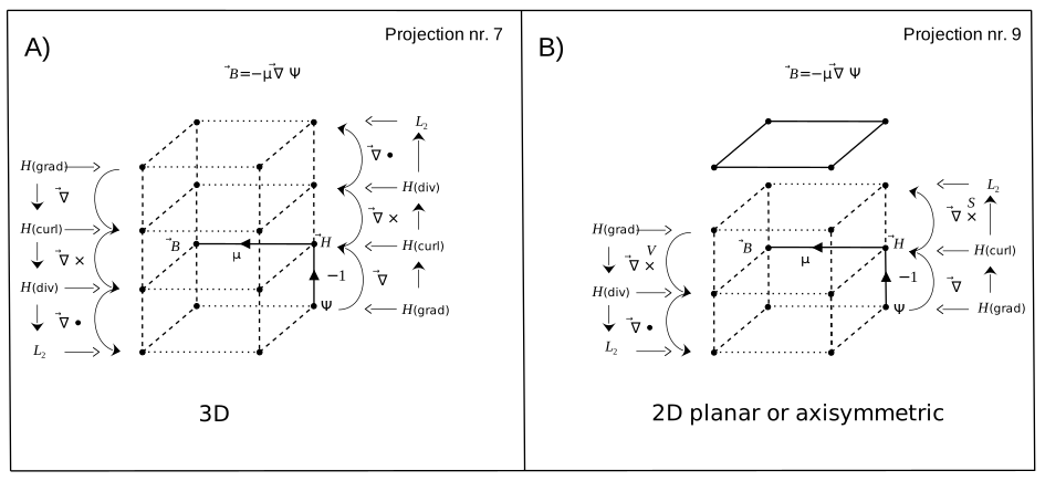
The total scalar magnetic potental, \(\Psi\), is assumed to be an output of an object of the class StaticScalarSolver::Solver. That is, \(\Psi\) is expressed as a linear combination of the shape functions of the FE_Q finite elements. In other words, \(\Psi\) is in the \(H(\text{grad})\) function space. This class template computes the magnetic field \(\vec{B}\) such that \(\vec{B}\) is expressed as a linear combination of the shape functions of the FE_RaviartThomas finite elements. That is, \(\vec{B}\) is in the \(H(\text{div})\) function space. In other words, this class template takes a scalar function \(\Psi\) from the \(H(\text{grad})\) function space, calculates its gradient, multiplies the gradient by \(-\mu\), and projects the result into \(H(\text{div})\) function space, which is a proper space for the magnetic field \(\vec{B}\). The operation of projection is illustrated by means of the Bossavit's diagrams below.

It is assumed that the object of the class StaticScalarSolver::Solver that yielded \(\Psi\) is still in the computer memory such that the triangulation, the degrees of freedom, and the handler of the degrees of freedom are accessible while \(\vec{B}\) is computed. An object of the StaticScalarSolver::ProjectPSItoB class template reuses the triangulation by creating an additional dof handler associated with the FE_RaviartThomas finite elements. That is, \(\vec{B}\) and \(\Psi\) share the same triangulation but are modeled by different finite elements: \(\vec{B}\) - by FE_RaviartThomas and \(\Psi\) - by FE_Q. In this disposition there are two DoFHandler objects associated with one Triangulation object. The algorithm walks synchronously through both DoFHandler objects and assembles the system matrix and the right-hand side. The algorithm utilizes the WorkStream technology of deal.II. The amount of threads used can be limited as the following

#include <deal.II/base/multithread_info.h>
 
MultithreadInfo::set_thread_limit(nr_threads_max);

It is also assumed that the object of the type StaticScalarSolver::TheCoefficient that was used to calculate \(\Psi\) is still in memory. The function implemented by this object is evaluated at the quadrature points and interpreted as permeability, \(\mu\), which is necessary ingredient for computing \(\vec{B}\), see above.

The output data are saved into a vtk file. The following data are saved:

The calculated magnetic field, \(\vec{B} = - \mu \vec{\nabla} \Psi\), under the name "VectorField".
The \(L^2\) and \(L^{\infty}\) error norms associated with the calculated magnetic field under the names "L2norm" and "LinftyNorm". One value per mesh cell is saved.
The exact solution projected onto \(H(\text{curl})\) function space is saved under the name "VectorFieldExact". The "VectorField" and "VectorFieldExact" are modeled by exactly the same finite elements, i.e., FE_RaviartThomas.

The "L2norm", "LinftyNorm", and "VectorFieldExact" are saved only if an exact solution is passed to the constructor. Moreover, "VectorFieldExact" is calculated and saved only if the input parameter project_exact_solution passed to the constructor equals true.

The user is supposed to derive an object from this class template. All usual computations, i.e., setup, assembling the linear system, etc., happen automatically.

Note

Application examples:

sld-i/ - Projection nr. 7 and projection nr. 9 (planar).

Definition at line 104 of file project_PSI_to_B.hpp.

Constructor & Destructor Documentation

◆ ProjectPSItoB()

template<int dim, int stage = 1>

StaticScalarSolver::ProjectPSItoB< dim, stage >::ProjectPSItoB	(	unsigned int	p,
		unsigned int	mapping_degree,
		const Triangulation< dim > &	triangulation_PSI,
		const DoFHandler< dim > &	dof_handler_PSI,
		const Vector< double > &	solution_PSI,
		std::string	fname = `"B"`,
		const Function< dim > *	exact_solution = `nullptr`,
		bool	axisymmetric = `false`,
		bool	print_time_tables = `false`,
		bool	project_exact_solution = `false`,
		bool	log_cg_convergence = `false`,
		bool	write_higher_order_cells = `false`
	)

inline

The only constructor.

Constructs the object and runs the calculations. That is, there is no need to call other functions such as run().

Parameters

[in]	p	- The degree of the FE_RaviartThomas finite elements.
[in]	mapping_degree	- The degree of the interpolating polynomials used for mapping. Setting it to 1 will do in the most of the cases. Note, that it makes sense to attach a meaningful manifold to the triangulation if this parameter is greater than 1.
[in]	triangulation_PSI	- Reference to the triangulation inside an object of the class StaticScalarSolver::Solver that has yielded the total scalar magnetic potential, \(\Psi\).
[in]	dof_handler_PSI	- Reference to the dof handler inside the class StaticScalarSolver::Solver that has yielded the total scalar magnetic potential, \(\Psi\).
[in]	solution_PSI	- Vector filled with the degrees of freedom that together with the shape functions of the FE_Q finite elements model the total scalar magnetic potential, \(\Psi\).
[in]	fname	- The name of the output files without extension.
[in]	exact_solution	- Points to an object that describes the exact solution to the problem. It is needed for calculating error norms. The exact solution object must exist in the computer memory at the time of calling this constructor.
[in]	axisymmetric	- If true, assumes that the problem is axisymmetric. In this case, of course, the problem must be two- dimensional.
[in]	print_time_tables	- If true, prints time tables on the screen.
[in]	project_exact_solution	- If true, projects the exact solution onto the space spanned by the Raviart-Thomas finite elements and saves the result into the output file next to \(\vec{B}\).
[in]	log_cg_convergence	- If true, logs convergence of the conjugate gradient solver into a file. The name of the file is generated by appending "_cg_convergence.csv" to fname.
[in]	write_higher_order_cells	- If false, the data is saved in the file fname.vtk. Higher-order cells are not saved. If true, the data is saved into fname.vtu file preserving the higher-order cells. In this case the file can be viewed with a help of Paraview version 5.5.0 or higher.

Definition at line 153 of file project_PSI_to_B.hpp.

The documentation for this class was generated from the following file:

static/shared/include/project_PSI_to_B.hpp

Public Member Functions

Detailed Description

template<int dim, int stage = 1> class StaticScalarSolver::ProjectPSItoB< dim, stage >

Constructor & Destructor Documentation

◆ ProjectPSItoB()

template<int dim, int stage = 1>
class StaticScalarSolver::ProjectPSItoB< dim, stage >